Overview
I trained an Explainable Boosting Machine (EBM) to predict the profitability of options trades. This was my first EBM experiment, intended to provide an additional entry condition for a strategy based on the variance risk premium (VRP). Before I could use it in the strategy, I needed to establish whether the model could make useful predictions. The AI model wasn't stable across seed values, so I developed the work to predict actionable signals such as variance of the market returns rather than absolute options prices.
The problem
The idea was to use information available before entering a trade to estimate a filter that would leave the remaining trades slightly more profitable on average. I was working towards an additional edge for a VRP strategy, but this model tried to predict trade profit directly. Realised and implied volatility were among its inputs; neither was the prediction target.
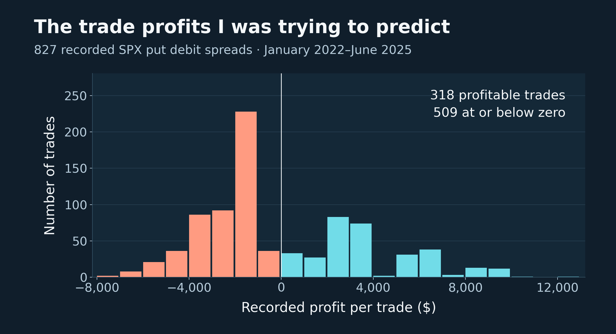
The training examples were SPX 0DTE put debit spreads, generally entered at about 15:15 and held to expiry that day at 16:00. The model therefore had to account for the direction and size of the remaining price move, the entry cost and the spread’s payoff. A good estimate of volatility alone wouldn’t necessarily tell it whether the put spread would make money.
What was achieved?
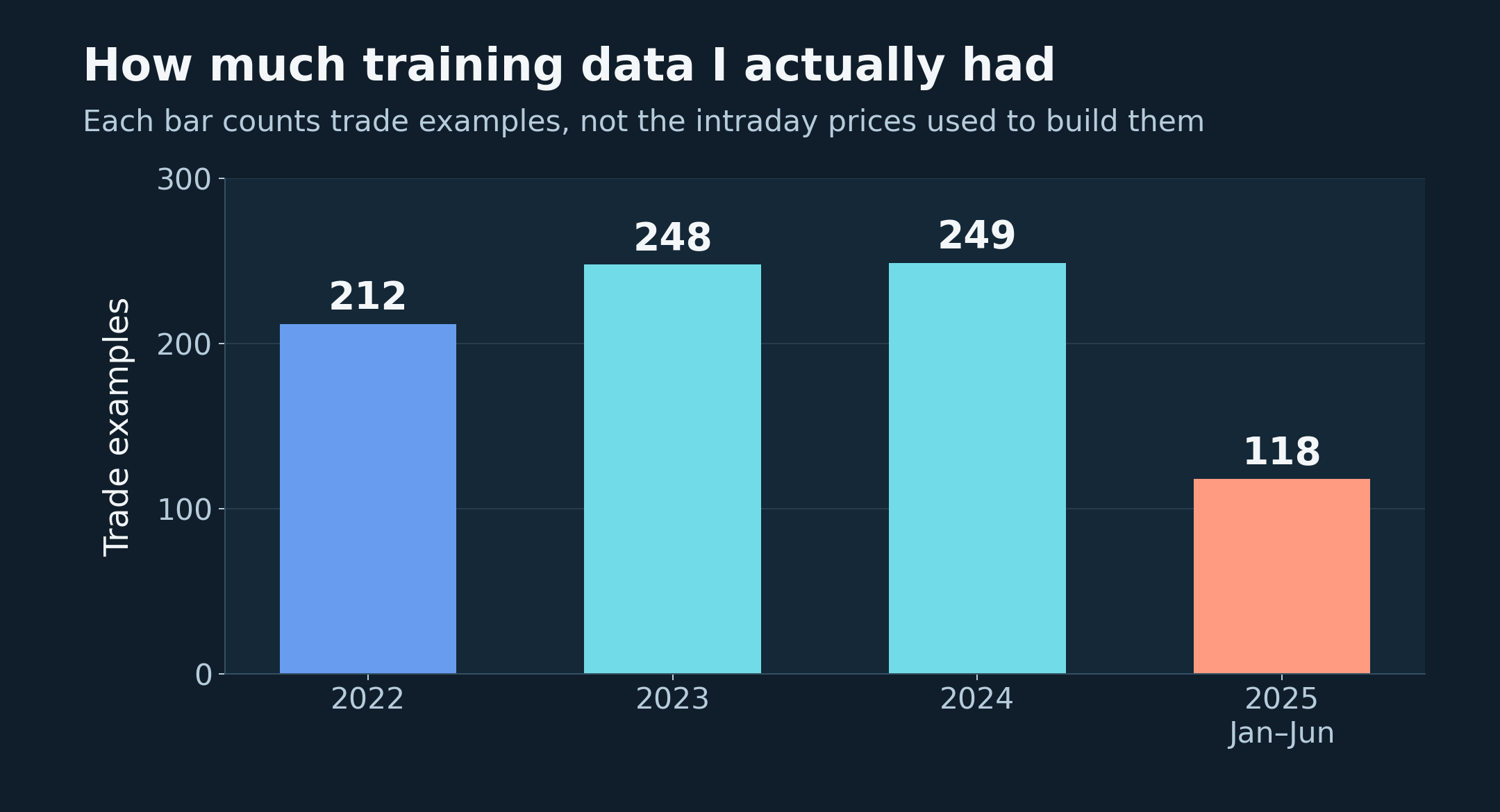
I assembled 827 trade examples from 2022 to the middle of 2025, with 27 input variables. I built the data processing and training scripts and produced graphs of the functions the model had learned. This made it possible to inspect how individual inputs were affecting the prediction.
I tried several training configurations, but the models were either too flexible or too restricted. Reducing the apparent overfit often left a model that didn’t learn enough to be useful. The experiment did not establish a reliable profit filter.
Technical implementation
I used Excel, DuckDB and Python for different parts of the data preparation. Excel was useful for inspecting and formatting intermediate data. I used Python scripts to calculate features from the intraday data, then DuckDB queries to join the separate feature tables by date and export the training CSVs using SQL.
The inputs covered price ranges, returns over different parts of the session, implied volatility at entry and changes in IV. I also calculated realised volatility and absolute movement from one-minute and five-minute prices, together with volume and VWAP measures and the trade’s maximum risk. This gave the model several descriptions of the same trading session.
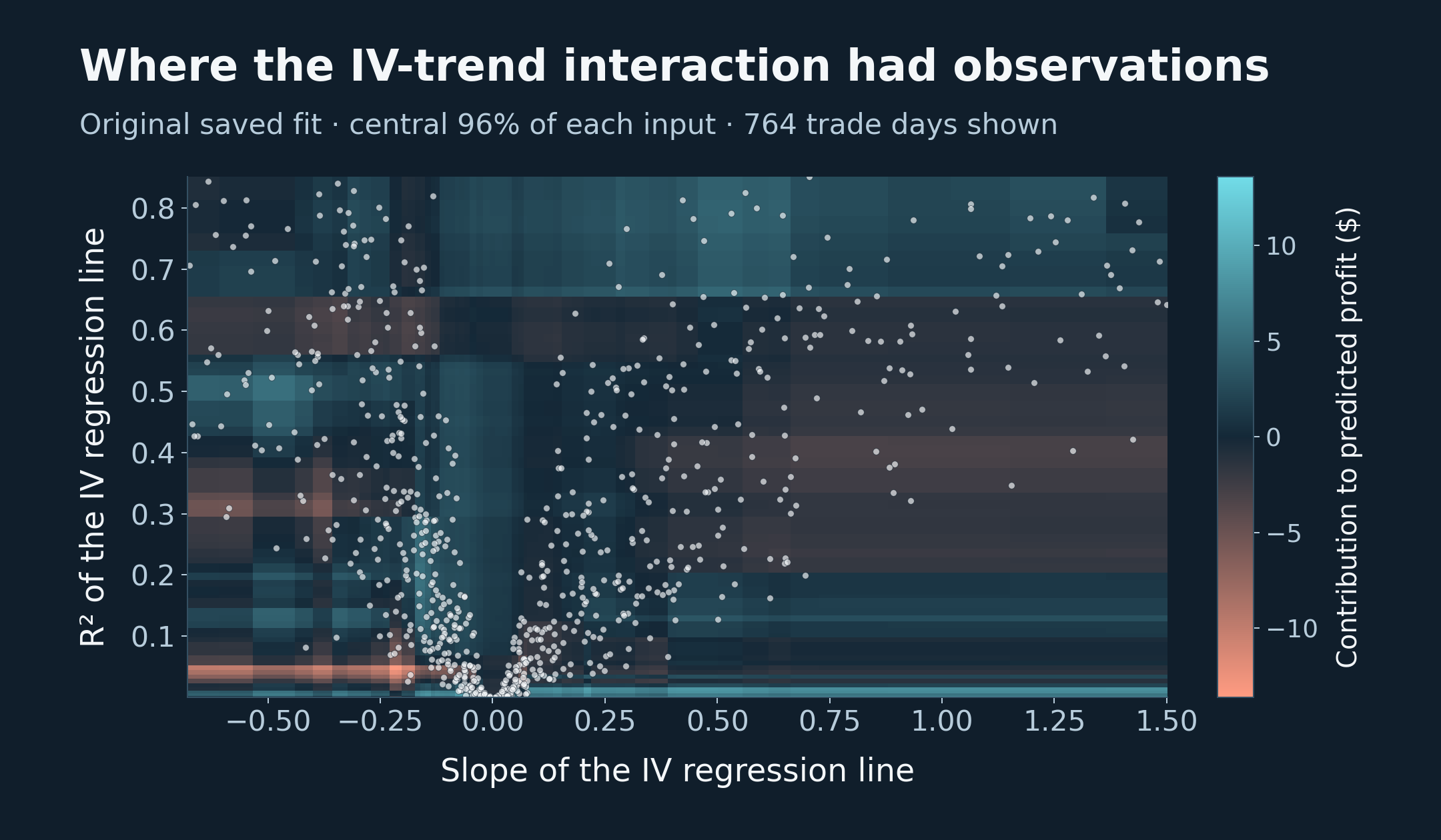
The first specification had 21 main effects and 9 paired interactions, giving 30 learned terms from the 27 variables. Six variables were only used in interactions. For example, I paired the slope of the IV regression line with its R², so that the model could consider the direction of the trend together with how closely the observations followed it. I did the same for price and volume trends.
I used InterpretML’s ExplainableBoostingRegressor with its default RMSE objective. With the identity link, the prediction was an intercept plus the contributions from the individual terms. I could inspect these as one-dimensional functions and two-dimensional interaction plots. At this stage I wasn’t comparing regression loss functions or experimenting with log links.
Why this did not work
There were too many flexible terms for the amount of training data. Hundreds of intraday prices still produced only one trade example for a day. Once those 827 examples were divided between different feature ranges and paired combinations, some regions had very little data behind them. Market conditions also persisted across days, so successive examples weren’t independent observations of entirely new conditions.
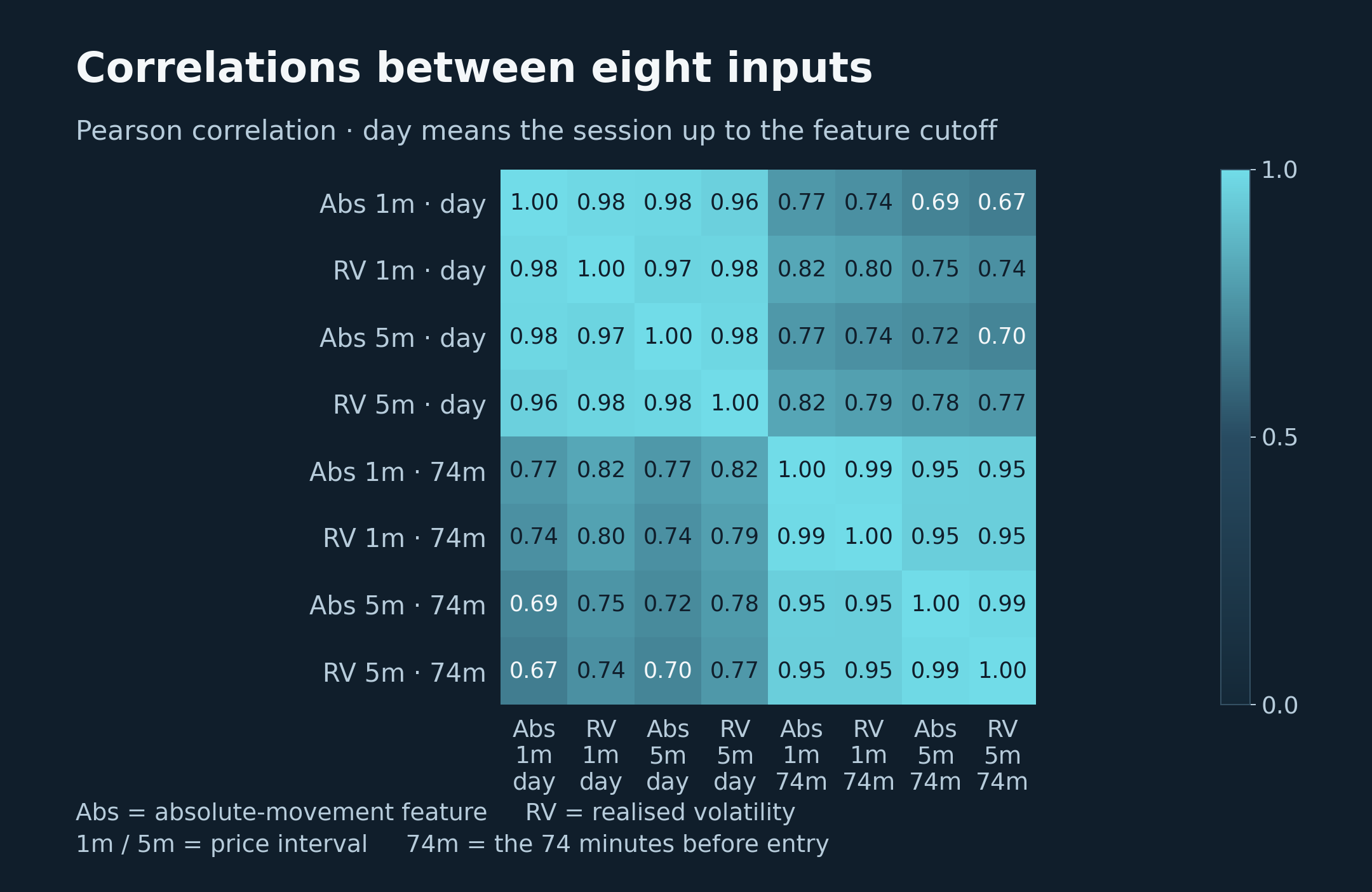
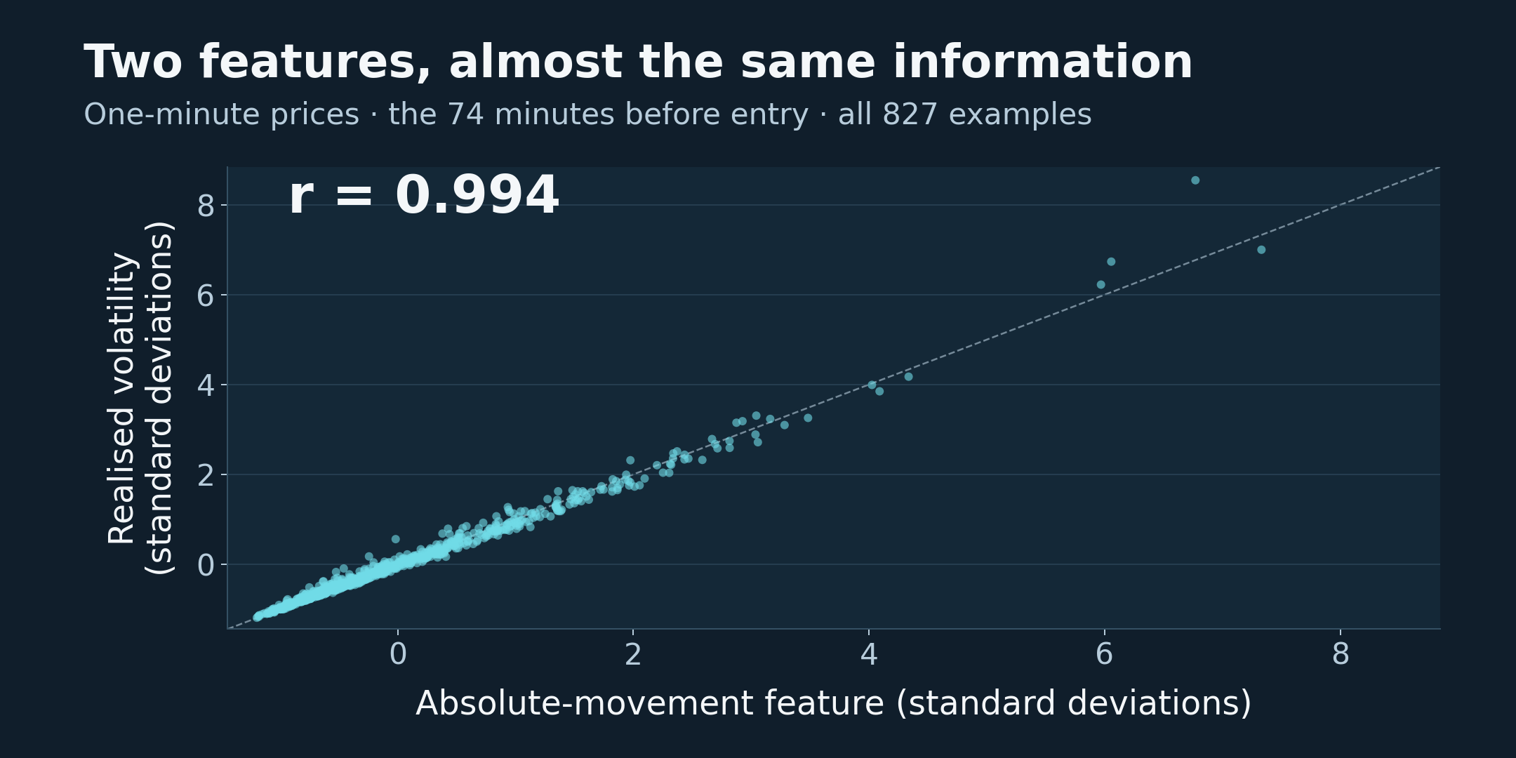
Many inputs were almost duplicates. In the original training data, the correlation between the one-minute absolute-movement measure and realised volatility over the 74-minute period before entry was about 0.994. Several other movement and volatility pairs were above 0.98. Adding these variables gave the model more ways to explain the same observations without adding much new information. It also made the contribution attributed to any one feature harder to trust.
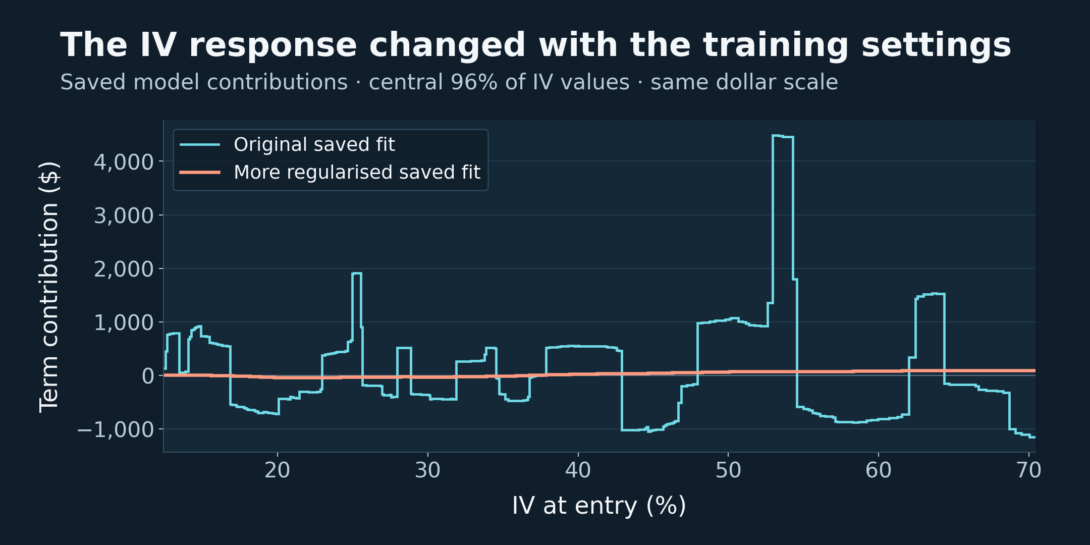
My initial training settings used one outer bag and disabled early stopping. It printed errors calculated on the data passed to fit, so those figures couldn’t establish how the model would perform on future trades. I later tried more bagging, smoothing and regularisation, as well as different bin counts, but didn’t find a stable fit.
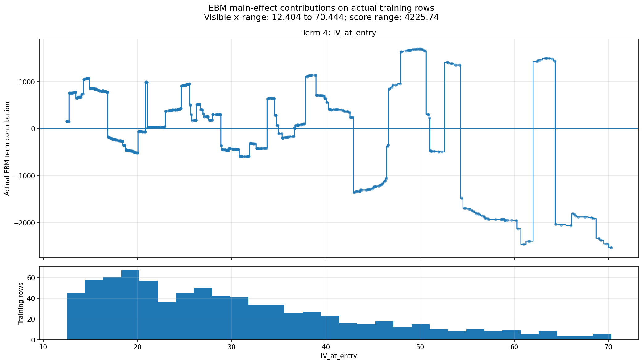
The saved graph below shows the contribution from IV at entry and the distribution of training examples. There are large changes in the contribution over small changes in IV, including regions with few observations. EBM functions are binned, so steps alone don’t prove overfit, but this was the sort of behaviour that needed to hold up on new data before I could use it.
The target was very difficult for the model to learn. Trade profit included the cost of buying options whose market prices already reflected expectations about future movement. The model needed to find something useful beyond that pricing. I underestimated how difficult this would be with a small dataset and largely overlapping market features
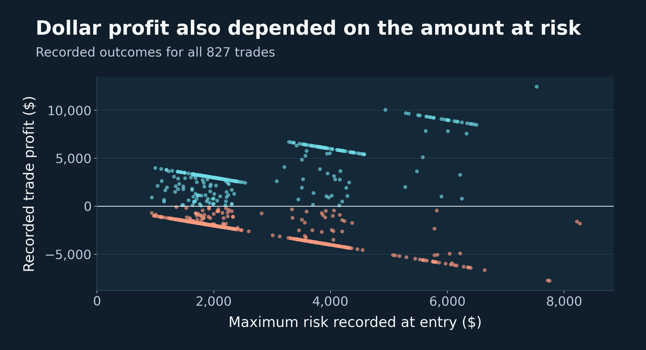
Profit also mixed the quality of the entry with the amount at risk and the eventual payoff. Large dollar errors could dominate squared-error training even when they didn’t identify the most useful entry rule. Conversely, a lower average prediction error wouldn’t necessarily improve the trades selected after costs.
What I would do differently
I would start with a much smaller set of inputs and a simple baseline, testing additions on a later validation period before committing to the final specification.
My later EBM work made me pay more attention to walk-forward testing, comparisons across random seeds and the number of observations supporting each learned function. I would choose the settings using the in sample period, then a walk forward on subsequent periods. I would also compare the strategy with and without the filter, including models for trading costs I’ve developed for other projects.
The later volatility models gave me a more specific prediction problem. Estimating the remaining realised variance and comparing it with the variance implied by options was closer to the VRP idea I was trying to use. It still required a separate test of whether the resulting entry condition improved the strategy.
Choice of loss function
For the original profit target, I would test pseudo-Huber loss alongside RMSE. It behaves approximately like squared error for small residuals and becomes closer to absolute error for large ones, reducing the influence of a few large errors.
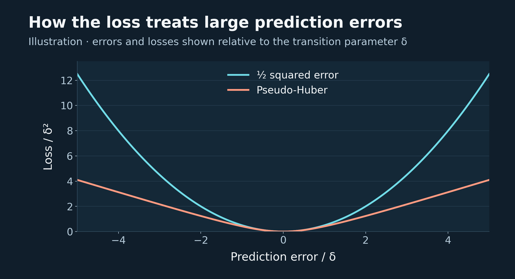
I wouldn’t assume it would be better. Squared-error loss is appropriate when the quantity I want is expected profit. Pseudo-Huber doesn’t generally estimate mean profit, and large gains and losses can be economically important. I would keep RMSE as the baseline and compare the forecasts and the trades selected on later data, including the largest losses.
Gamma deviance and a log link, which I used in later volatility work, wouldn’t directly suit this original target. Profit can be negative, Gamma deviance requires positive targets, and a log link forces the predicted value to be positive. If I changed the task to predicting the probability of a profitable trade, log loss would be appropriate, but the win probability would still need to be considered alongside the size of wins and losses.
Changing the loss could have made training less sensitive to large residuals. It wouldn’t have supplied the missing data or shown that the original inputs contained a repeatable trading edge.